Having your own cloud does not mean you are out of the resource planning business, but it does make the job a lot easier. If you collect the right data, with the application of some well understood statistical practices, you can break the work down into two different tasks: supporting workload volatility and resource planning.
If the usage of our applications was changing in a predictable fashion, resource planning would be easy. But that’s not always the case, and volatility can make it very difficult to tell what is a short term change and what is part of a long term trend. Here are some steps to help you prioritize systems for consolidation, get ahead of future capacity problems, and understand long term trends to assist in purchasing behaviors. Our example is with data extracted from Red Hat’s ManageIQ cloud management software.
Usually, we collect and see our performance over X periods of time, where X is a small number and we don’t get much insight. More data points are help, but require a lot of storage. ManageIQ natively provides data rollup of metrics, to provide a great balance between the two. Since we want to compare short term to long term for trends, we lose little using the rollup data.
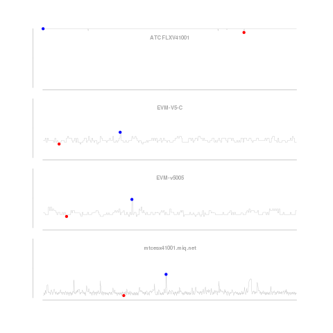
 Our graphs look at the CPU utilization history of four systems. The first graph looks only at the short term data, smoothed (using a process similar to the one described here) over one minute intervals. We smooth the data to reduce the impact of intra-period volatility on our predictions. The method described corrects for “seasonality” within the periods, e.g. CPU utilization on Mondays could be predictably higher than on Tuesdays as customers come back to work and get things done they could not over the weekend. The blue dot is the highest utilization, and red, the lowest over the period. Continue reading “Load Volatility and Resource Planning for your Cloud” →

