 Usage is over threshold, unleash the kraken!
Short run peaks are perfect for automated elasticity: the unpredictable consumption that we stay up late worrying about fulfilling. But, short run peaks can be difficult to tease out from expected variation within the period: seasonality. Using the open source statistical package R, we can separate and look at both.
Our example will be watching the one, five, and fifteen minute load averages from my laptop over the past few work days, measured at 10 second intervals. (Also in the file is the CPU temp). Taking the test across the one minute load averages from the data, here’s what we’d like to see:
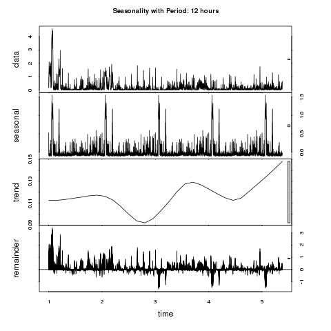 The four graphs indicate the raw data, seasonal adjustments, trend adjusted for seasonality, and the remainder (data – seasonality). The time scale is in units of 12 hours, as suggested by the title of the graph.
Determining the right length of period to measure is a combination of method and reason. I tested all period lengths from 1 to 24 hours, using the code below. The optimal period suggested by the code was 13 hours. As 12 hours makes more sense in terms of work hours, and the difference was minimal, I have elected to use 12 hours. Running the same across five and fifteen minute load averages, as well as temperature we see suggested period of 15, 11, and 1 hours respectively.
From the trend chart, we see a distinct and pronounced upward trend in the one minute load average. This is what you take long-term action on.
Graph comment: To the very right side of that graph is a grey rectangle. It’s a visual clue to the scale of the curve relative to the others in the collection.
R Code
w <- data.frame(0,0,0)

names(w) <- c("period", "mean", "stdev")

# 360 = 1 hour of 10 second intervals

# if you want to look for longer periods (days, weeks, months, etc.),

# change the second field in the seq function

for ( win in seq(360,360*24,360) ) {

myts <- ts(csv$fifteen, names=csv$date, frequency=win)

fitR <- stl(myts, s.window="period",robust=T)

w <- rbind(w, c(win, mean(fitR$weights), sd(fitR$weights)))

}

w[1,] <- NA

w <- w[!is.na(w$period),]

period <- w[w$mean == min(w$mean),]$period

myts <- ts(csv$fifteen, names=csv$date, frequency=period)

fitR <- stl(myts, s.window="period",robust=T)

print(paste("Optimal value of", period/360, "hours"))

plot(fitR, main=paste("Seasonality with Period:", period/360, "hours"))